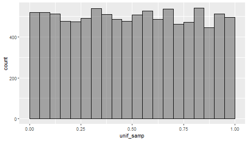
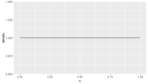
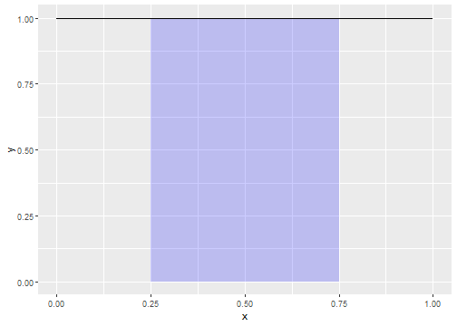
class: center, middle, inverse, title-slide # Lecture 6 ## Random Variables ### JMG ### MATH 204 ### Thursday, September 16 --- # Learning Objectives In this lecture, we will - Examine the most important concepts related to our study of random variables. -- - Recall from the last lecture that we introduced the notion of a random variable, that is, something that assigns a numerical value to events from a random process. -- - We typically denote random variables by capital letters at the end of the alphabet such as `\(X\)`, `\(Y\)`, or `\(Z\)`. -- - Our primary goal is to study methods that allow us to better understand the distribution of a random variable. -- - Specifically, we will cover expectation, variance, discrete and continuous distributions, and some common random variables and their distributions. See textbook sections 3.4, 3.5, 4.1, 4.2, and 4.3. --- # Random Variable Distributions - If a random variable has only a very small number of outcomes, then we can simply list its distribution. -- - For example, reconsider the process of rolling two six-sided dice. Let `\(X\)` be the random variable that records the sum of the values shown by the two dice. Then the distribution for `\(X\)` is <table class="table" style="margin-left: auto; margin-right: auto;"> <tbody> <tr> <td style="text-align:left;"> Dice sum </td> <td style="text-align:left;"> X=2 </td> <td style="text-align:left;"> X=3 </td> <td style="text-align:left;"> X=4 </td> <td style="text-align:left;"> X=5 </td> <td style="text-align:left;"> X=6 </td> <td style="text-align:left;"> X=7 </td> <td style="text-align:left;"> X=8 </td> <td style="text-align:left;"> X=9 </td> <td style="text-align:left;"> X=10 </td> <td style="text-align:left;"> X=11 </td> <td style="text-align:left;"> X=12 </td> </tr> <tr> <td style="text-align:left;"> Probability </td> <td style="text-align:left;"> 1/36 </td> <td style="text-align:left;"> 2/36 </td> <td style="text-align:left;"> 3/36 </td> <td style="text-align:left;"> 4/36 </td> <td style="text-align:left;"> 5/36 </td> <td style="text-align:left;"> 6/36 </td> <td style="text-align:left;"> 5/36 </td> <td style="text-align:left;"> 4/36 </td> <td style="text-align:left;"> 3/36 </td> <td style="text-align:left;"> 2/36 </td> <td style="text-align:left;"> 1/36 </td> </tr> </tbody> </table> -- - We can compute probability values associated with `\(X\)` such as `$$P(X=3) = \frac{2}{36}=\frac{1}{18}$$` or `$$P(X <= 5) = \frac{1}{36}+\frac{2}{36}+\frac{3}{36}+\frac{4}{36}=\frac{10}{36}=\frac{5}{18}$$` --- # Tossing a Coin - Consider the random process of tossing a coin where the probability of landing heads is a number `\(p\)`. Let `\(X\)` be the random variable that counts the number of heads after a single toss. -- - Construct the probability distribution for `\(X\)`. Note that the only possible outcomes for `\(X\)` is 0 or 1. -- - Obviously `\(P(X=1) = p\)`. -- - By the complement rule, we must have `\(P(X=0) = 1 - p\)`. Therefore, <table class="table" style="margin-left: auto; margin-right: auto;"> <tbody> <tr> <td style="text-align:left;"> Num Heads </td> <td style="text-align:left;"> X=0 </td> <td style="text-align:left;"> X=1 </td> </tr> <tr> <td style="text-align:left;"> Probability </td> <td style="text-align:left;"> 1-p </td> <td style="text-align:left;"> p </td> </tr> </tbody> </table> --- # Summaries for Random Variable Distributions - In cases where it is not easy to completely write down the probability distribution for a random variable, it is useful to be able to characterize the distribution. -- - The two most common characteristics we consider for the distribution of a random variable are its **expectation** or expected value, and its **variance**. -- - We will discuss expectation first. --- # Discrete Vs. Continuous Random Variables - Before we define the expectation of a random variable, it is helpful to distinguish two types of random variables. -- - A random variable `\(X\)` is called **discrete** if its outcomes form a discrete set. - A set is discrete if it can be labeled by the whole numbers 1, 2, 3, ... -- - For example, the random variable that adds the values after a roll of two six-sided dice is a discrete random variable. Additionally, the random variable that counts the number of heads after tossing a coin 10 times is a discrete random variable. -- - Later we will describe continuous random variables. However, it's important to note that there are random variables that are neither discrete or continuous. --- # Expectation - Expectation, or the expected value of a random variable `\(X\)` measures the average outcome for `\(X\)`. We typically denote the expectation of `\(X\)` by `\(E(X)\)`, or sometimes by `\(\mu\)`. -- - The expected value of a discrete random variable `\(X\)` is the sum of the products of its outcomes times its probability values. -- - Mathematically, `$$E(X) = x_{1}P(X=x_{1}) + x_{2}P(X=x_{2}) + \cdots + x_{n}P(X=x_{n})$$` -- - For example, if `\(X\)` is the random variable that adds the values after a roll of two six-sided dice, then $$ `\begin{align*} E(X) &= 2\frac{1}{36}+3\frac{2}{36}+4\frac{3}{36}+5\frac{4}{36}+6\frac{5}{36} \\ & +7\frac{6}{36}+8\frac{5}{36}+9\frac{4}{36}+10\frac{3}{36}+11\frac{2}{36}+12\frac{1}{36} \\ &= \frac{245}{36} \approx 6.8 \end{align*}` $$ --- # Considering Data - The following shows the first few rows from data collected after repeatedly tossing two dice 5,000 times and adding up their values after each toss: ``` ## # A tibble: 6 x 3 ## die_1 die_2 sum ## <int> <int> <int> ## 1 6 2 12 ## 2 2 4 4 ## 3 6 5 12 ## 4 2 4 4 ## 5 2 6 4 ## 6 6 4 12 ``` -- - Let's compute the mean for the sum variable: ``` ## [1] 7.0548 ``` -- - The point is that expected value is to random variables what the mean is to data. -- - That is, if we take a very large number of samples from a random variable and compute the sample mean, then this will give us an accurate (but not exact) estimate for the expected value. --- # Another Expectation Example - Suppose we let `\(X\)` be the random variable that counts the number of heads after a single toss of a coin with probability of getting heads `\(p\)`. -- - Then, `$$E(X) = 1 \cdot p + 0 \cdot (1-p) = p$$` -- - If our coin is fair, then `\(p=\frac{1}{2}\)` and `\(E(X) = \frac{1}{2}\)`. -- - Here's the mean of 1,000 samples from this random variable (number of heads for a fair coin): ``` ## [1] 0.527 ``` --- # Basic Properties of Expectation - The expected value satisfies some important properties, among the most important are: -- - If we multiply a random variable `\(X\)` by a number `\(a\)`, and then add another number `\(b\)`, then we can compute the expected value in either of two ways and get the same answer. Mathematically, `$$E(aX + b) = aE(X) + b.$$` -- - If we have two random variables `\(X\)` and `\(Y\)`, and we multiply them each by a different number and add the result, then we can compute the expected value in either of two ways and get the same answer. Mathematically, `$$E(aX+bY) = aE(X) + bE(Y)$$` -- - The previous result extends to any number of random variables. In particular, `$$E(X_{1} + X_{2} + \cdots + X_{n}) = E(X_{1}) + E(X_{2}) + \cdots + E(X_{n})$$` --- # Examples Working with Expectation - We will take a pause from the slides to work out some examples together. --- # Variance of a Random Variable - We have seen that expected value is to random variables what the mean is to data. What is the analog of the sample variance of data for a random variable? -- - The answer is the **variance** of a random variable. If `\(X\)` is a random variable and `\(\mu\)` is its expected value, then the variance of `\(X\)` is `$$\text{Var}(X) = E((X - \mu)^2)$$` - The standard deviation of a random variable `\(X\)` is the square root of its variance `\(\text{sd}(X) = \sqrt{\text{Var}(X)}\)`. -- - It is helpful to know that if `\(a\)` and `\(b\)` are numbers and if `\(X\)` is a random variable, then `$$\text{Var}(aX + b) = a^2\text{Var}(X)$$` --- # Considering Data for Variance - You can take it on faith that if `\(X\)` is the random variable that returns the number of heads after a single toss of a fair coin, then `\(\text{Var}(X) = \frac{1}{4}=0.25\)`. Let's see how this compares with the sample variance of some data: -- - The sample variance after 1,000 sample tosses is ``` ## [1] 0.2502142 ``` --- # Examples Working with Variance - We will take a pause from the slides to work out some examples together. --- # Famous Distributions and Their Properties - Now that we have covered the principal concepts regarding random variables, we introduce some famous types of random variables and describe their distributions. -- - We begin with some famous discrete distributions. -- - Bernoulli, Geometric, and Binomial -- - Then we discuss continuous random variables and the most famous continuous distribution, the normal distribution. --- # Bernoulli Random Variable A **Bernoulli random variable** (section 4.2.1) is a random variable `\(X\)` corresponding to a random process with exactly two possible outcomes typically labeled "success" and "failure", a so-called Bernoulli trial. We define `\(X\)` by counting the number of successes after a single trial so that `\(X=1\)` (for a success) and `\(X=0\)` for failure. -- - If `\(p\)` is the probability of success, then the probability distribution of `\(X\)` is <table class="table" style="margin-left: auto; margin-right: auto;"> <tbody> <tr> <td style="text-align:left;"> Num Successes </td> <td style="text-align:left;"> X=0 </td> <td style="text-align:left;"> X=1 </td> </tr> <tr> <td style="text-align:left;"> Probability </td> <td style="text-align:left;"> 1-p </td> <td style="text-align:left;"> p </td> </tr> </tbody> </table> -- - If `\(X\)` is a Bernoulli random variable, then `$$\mu=E(X) = p, \ \ \text{ and } \ \ \sigma^2=\text{Var}(X) = p(1-p)$$` -- - Note that the flip of a coin can be modeled by a Bernoulli random variable if we think of tossing heads as a success and if the probability of tossing heads is `\(p\)`. --- # Bernoulli Examples - We take a break from the slides to work out some examples related to Bernoulli random variables. --- # The Geometric Distribution The geometric distribution is used to describe how many trials it takes to observe a success. -- - Suppose we conduct a sequence of `\(n\)` independent Bernoulli trials with probability of success `\(p\)`. What is the probability that it takes `\(n\)` trials to obtain the first success? -- - Let `\(A\)` be the event that the first success occurs on the `\(n\)`-th trial. Then `\(A\)` can be realized as the event `\(A = F_{1} \text{ and } F_{2} \text { and } \cdots \text{ and }F_{n-1} \text{ and }S_{1}\)`, where and `\(F\)` corresponds to a failure event and an `\(S\)` corresponds to a success event. Since there are all independent, we have `$$P(A) = P(F_{1})P(F_{2})\cdots P(F_{n-1})P(S_{1}) = (1-p)^{n-1}p$$` -- - If `\(X\)` is a random variable with a geometric distribution, then `$$\mu=E(X) = \frac{1}{p}, \ \ \text{ and }\ \ \sigma^{2}=\text{Var}(X) = \frac{1-p}{p^2}$$` --- # Geometric Distribution Examples - We take a break from the slides to work out some examples related to Geometric random variables. --- # The Binomial Distribution - The binomial distribution is used to describe the number of successes in a fixed number of trials. This is different from the geometric distribution, which describes the number of trials we must wait before we observe a success. -- - For a binomial distribution, -- - The number of trials, `\(n\)`, is fixed. -- - The trials are independent. -- - Each trial outcome can be classified as a success or failure. -- - The probability of a success, `\(p\)`, is the same for each trial. --- # Mathematics of the Binomial Distribution - Suppose the probability of a single trial being a success is `\(p\)`. Then the probability of observing exactly `\(k\)` successes in `\(n\)` independent trials is given by $$ `\begin{align*} {n\choose k}p^k(1-p)^{n-k} &= \frac{n!}{k!(n-k)!}p^k(1-p)^{n-k} \end{align*}` $$ -- - The mean, variance, and standard deviation of the number of observed successes are $$ `\begin{align*} \mu &= np &\sigma^2 &= np(1-p) &\sigma&= \sqrt{np(1-p)} \end{align*}` $$ --- # Binomial Distribution Examples - We take a break from the slides to work out some examples related to Binomial random variables. -- - This video is also recommended: <div class="vembedr" align="center"> <div> <iframe src="https://www.youtube.com/embed/tKmyzhvgudw" width="533" height="300" frameborder="0" allowfullscreen=""></iframe> </div> </div> --- # Continuous Distributions - Each of the Bernoulli, Geometric, and Binomial distributions are discrete. -- - We will also be interested in **continuous** random variables. -- - Continuous random variables are tricky to define precisely. Roughly, a random variable `\(X\)` is a continuous random variable if its outcomes are continuous numerical values. -- - Consider for example a random variable `\(X\)` whose outcomes can be any real number in the interval `\([0,1]\)` and with each outcome equally likely. Such a random variable is said to follow a uniform distribution on `\([0,1]\)`. -- - If `\(x\)` is any real number in `\([0,1]\)`, then `\(P(X=x) = 0\)`. However, if `\(a,b\)` are any two real numbers in `\([0,1]\)` with `\(a\leq b\)`, then `\(P(a \leq X \leq b) = b - a\)`. -- - The quantity `\(P(a \leq X \leq b)\)` is interpreted as the probability of randomly selecting any real number in `\([0,1]\)` that lies between `\(a\)` and `\(b\)`. --- # Samples from a Uniform Distribution The following plot shows a histogram of 10,000 random samples from a uniform distribution on `\([0,1]\)`: -- <!-- --> -- - If you had to guess, what do you think are the expected value and standard deviation for a uniform random variable on `\([0,1]\)`? --- # Uniform Distribution: Density - The following plot shows the **probability density function** for a uniformly distributed random variable on `\([0,1]\)`: <!-- --> -- - Pick two values `\(a\)` and `\(b\)` that lie within `\([0,1]\)`. Then the **area** that falls under the density function and between the lines `\(x=a\)` and `\(x=b\)` corresponds to the probability that a random variable `\(X\)` uniform on `\([0,1]\)` takes values between `\(a\)` and `\(b\)`. --- # Are Under a Density Function - The following shaded rectangle shows the area under the density function for a uniform distribution on `\([0,1]\)` between 0.25 and 0.75. This area represents the probability that a value for a random variable `\(X\)` uniformly distribution on `\([0,1]\)` falls between 0.25 and 0.75. Thus, `\(P(0.25 \leq X \leq 0.75) = 0.75 - 0.25 = 0.5\)`. <!-- --> --- # General Continuous Distributions - Hopefully, the last few slides provide intuition for the following facts: -- - If `\(X\)` is a random variable, and there is a continuous function `\(f\)` such that `\(P(a \leq X \leq b) = \text{area under graph of } f\)` between `\(a\)` and `\(b\)`, then `\(X\)` is a continuous random variable with probability density function `\(f\)`. -- - Note that for any density function `\(f\)`, we require that the total area under the graph of `\(f\)` is 1. --- # The Normal Distribution - Perhaps the most famous and most important continuous distribution is the so-called **normal distribution.** This will be the topic of our next lecture. -- - To prepare for the next lecture, please watch the following video: <div class="vembedr" align="center"> <div> <iframe src="https://www.youtube.com/embed/S_p5D-YXLS4" width="533" height="300" frameborder="0" allowfullscreen=""></iframe> </div> </div> --- # R Commands for Distributions - We now show how you can use R to work with the distributions we have introduced so far. -- - Here is what you need to know: - Each distribution has a short hand name such `binom`, `geom`, `unif`, or `norm`. -- - Each distribution has four functions associated with it. For example, the four functions associated with `binom` are - `rbinom` - draws random samples from a binomial random variable -- - `dbinom` - implements the probability function for a binomial random variable -- - `pbinom` & `qbinom ` which implement the distribution function and quantile function respectively for a binomial random variable. We have not really discussed the concepts related to these functions at this point. -- - Let's go to R together and see how these all work.