R Commands for MATH 204
JMG
Some Useful R Commands
This notebook illustrates some R commands that relate directly to the statistical concepts covered in MATH 204 Introduction to Statistics. The presentation is terse and there is little discussion on how to interpret results as these details are covered in lectures.
Loading Packages
It is necessary to load any package (other than base R) that contains commands that we want to use. Note that these packages have to be installed before they can be loaded. One can install packages using the “Packages” tab and then clicking the “Install” icon.
# load packages
library(tidyverse)
library(openintro)
library(ggformula)
library(ggmosaic)
library(broom)
library(GGally)
library(skimr)
Here is a brief overview on each of the packages we have loaded:
tidvyversecontains commands for working with data frames and creating plots withggplot,openintrois an R package that is associated with our textbook OpenIntro Statistics. Mostly it just contains data sets.ggformula,ggmosaic, andGGallyeach add enhanced plotting capabilities,broomhas commands that help clean up output from linear models,skimrcontains a command calledskimthat prints out a nice data summary.
Now that we’ve loaded our packages, we can import some data.
Load the Data
Here we load some data, the EPA 2021 vehicle data.
# load data
my_data <- read.csv("epa2021data.csv")
# if you don't have the data file, uncomment and use:
#my_data <- epa2021
This data contains vehicle information from the EPA for 2021. The size of this data set is reported by the following command:
dim(my_data)## [1] 1108 28We see that there are 1108 observations (rows) and 28 variables (columns).
It is a good idea to try to learn more about our data set. One
helpful command along these lines is the summary command
that prints out summary statistics for each variable in the data
set.
summary(my_data)## model_yr mfr_name division carline
## Min. :2021 Length:1108 Length:1108 Length:1108
## 1st Qu.:2021 Class :character Class :character Class :character
## Median :2021 Mode :character Mode :character Mode :character
## Mean :2021
## 3rd Qu.:2021
## Max. :2021
## mfr_code model_type_index engine_displacement no_cylinders
## Length:1108 Min. : 1.0 Min. :1.000 Min. : 3.000
## Class :character 1st Qu.: 40.0 1st Qu.:2.000 1st Qu.: 4.000
## Mode :character Median :114.0 Median :3.000 Median : 6.000
## Mean :259.4 Mean :3.125 Mean : 5.604
## 3rd Qu.:507.0 3rd Qu.:3.800 3rd Qu.: 6.000
## Max. :999.0 Max. :8.000 Max. :16.000
## transmission_speed city_mpg hwy_mpg comb_mpg
## Length:1108 Min. : 8.00 Min. :13.0 Min. :10.00
## Class :character 1st Qu.:17.00 1st Qu.:23.0 1st Qu.:19.00
## Mode :character Median :20.00 Median :27.0 Median :22.50
## Mean :20.89 Mean :27.3 Mean :23.29
## 3rd Qu.:23.00 3rd Qu.:31.0 3rd Qu.:26.00
## Max. :58.00 Max. :60.0 Max. :59.00
## guzzler air_aspir_method air_aspir_method_desc transmission
## Length:1108 Length:1108 Length:1108 Length:1108
## Class :character Class :character Class :character Class :character
## Mode :character Mode :character Mode :character Mode :character
##
##
##
## transmission_desc no_gears trans_lockup trans_creeper_gear
## Length:1108 Min. : 1.000 Length:1108 Length:1108
## Class :character 1st Qu.: 6.000 Class :character Class :character
## Mode :character Median : 8.000 Mode :character Mode :character
## Mean : 7.501
## 3rd Qu.: 8.000
## Max. :10.000
## drive_sys drive_desc fuel_usage fuel_usage_desc
## Length:1108 Length:1108 Length:1108 Length:1108
## Class :character Class :character Class :character Class :character
## Mode :character Mode :character Mode :character Mode :character
##
##
##
## class car_truck release_date fuel_cell
## Length:1108 Length:1108 Length:1108 Length:1108
## Class :character Class :character Class :character Class :character
## Mode :character Mode :character Mode :character Mode :character
##
##
## One benefit of the summary command is that it helps us to identify
the type of each variable. The glimpse command from the
pillar package (which is installed as part of
tidyverse) is also helpful in this regard.
pillar::glimpse(my_data)## Rows: 1,108
## Columns: 28
## $ model_yr <int> 2021, 2021, 2021, 2021, 2021, 2021, 2021, 2021, …
## $ mfr_name <chr> "Honda", "aston martin", "aston martin", "Volksw…
## $ division <chr> "Acura", "Aston Martin Lagonda Ltd", "Aston Mart…
## $ carline <chr> "NSX", "Vantage Manual", "Vantage V8", "R8", "R8…
## $ mfr_code <chr> "HNX", "ASX", "ASX", "VGA", "VGA", "VGA", "VGA",…
## $ model_type_index <int> 39, 5, 4, 5, 7, 6, 8, 73, 352, 350, 75, 76, 104,…
## $ engine_displacement <dbl> 3.5, 4.0, 4.0, 5.2, 5.2, 5.2, 5.2, 2.0, 3.0, 2.0…
## $ no_cylinders <int> 6, 8, 8, 10, 10, 10, 10, 4, 6, 4, 16, 16, 8, 12,…
## $ transmission_speed <chr> "Auto(AM-S9)", "Manual(M7)", "Auto(S8)", "Auto(A…
## $ city_mpg <int> 21, 14, 18, 13, 14, 13, 14, 23, 22, 25, 9, 8, 15…
## $ hwy_mpg <int> 22, 21, 24, 20, 23, 20, 23, 31, 30, 32, 14, 13, …
## $ comb_mpg <int> 21, 17, 20, 16, 17, 16, 17, 26, 25, 28, 11, 10, …
## $ guzzler <chr> "N", "N", "N", "Y", "Y", "Y", "Y", "N", "N", "N"…
## $ air_aspir_method <chr> "TC", "TC", "TC", NA, NA, NA, NA, "TC", "TC", "T…
## $ air_aspir_method_desc <chr> "Turbocharged", "Turbocharged", "Turbocharged", …
## $ transmission <chr> "AMS", "M", "SA", "AMS", "AMS", "AMS", "AMS", "A…
## $ transmission_desc <chr> "Automated Manual- Selectable (e.g. Automated Ma…
## $ no_gears <int> 9, 7, 8, 7, 7, 7, 7, 7, 8, 8, 7, 7, 8, 7, 7, 7, …
## $ trans_lockup <chr> "Y", "N", "Y", "N", "N", "N", "N", "N", "Y", "Y"…
## $ trans_creeper_gear <chr> "N", "N", "N", "N", "N", "N", "N", "N", "N", "N"…
## $ drive_sys <chr> "A", "R", "R", "A", "R", "A", "R", "A", "R", "R"…
## $ drive_desc <chr> "All Wheel Drive", "2-Wheel Drive, Rear", "2-Whe…
## $ fuel_usage <chr> "GPR", "GP", "GP", "GPR", "GPR", "GPR", "GPR", "…
## $ fuel_usage_desc <chr> "Gasoline (Premium Unleaded Required)", "Gasolin…
## $ class <chr> "Two Seaters", "Two Seaters", "Two Seaters", "Tw…
## $ car_truck <chr> "car", "car", "car", "car", "car", "car", "car",…
## $ release_date <chr> "2021-02-01T00:00:00Z", "2020-08-10T00:00:00Z", …
## $ fuel_cell <chr> "N", "N", "N", "N", "N", "N", "N", "N", NA, NA, …The next step in a data analysis is to conduct a so-called exploratory data analysis (EDA). This allows us to assess the data for any problems and also helps to suggest what types of statistical or analytical questions can be asked and/or answered.
The first steps in EDA are to compute summary statistics for variables of interest and to build appropriate summary visualizations.
Summary Stats for a Numerical Variable
For example, the comb_mpg variable (combined mileage) is
a continuous numerical variable so it makes sense to compute its mean,
median, standard deviation, and variance.
(comb_mpg_mean <- mean(my_data$comb_mpg))## [1] 23.2852(comb_mpg_median <- median(my_data$comb_mpg))## [1] 22.5(comb_mpg_sd <- sd(my_data$comb_mpg))## [1] 6.445931(comb_mpg_var <- var(my_data$comb_mpg))## [1] 41.55002Visual Summaries for Numerical Variables
Histograms and boxplots are appropriate ways to provide a visual summary for a numerical variable. The following plotting commands illustrate some of the ways in which such plots can be obtained.
gf_histogram(~comb_mpg,data=my_data)
Let’s change the number of bins and also add color to show where the bins are.
gf_histogram(~comb_mpg,data=my_data,bins=25,color="black")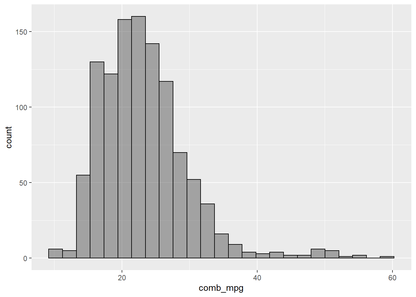
A boxplot is another way to visualize numerical data.
gf_boxplot(~comb_mpg,data=my_data) + coord_flip()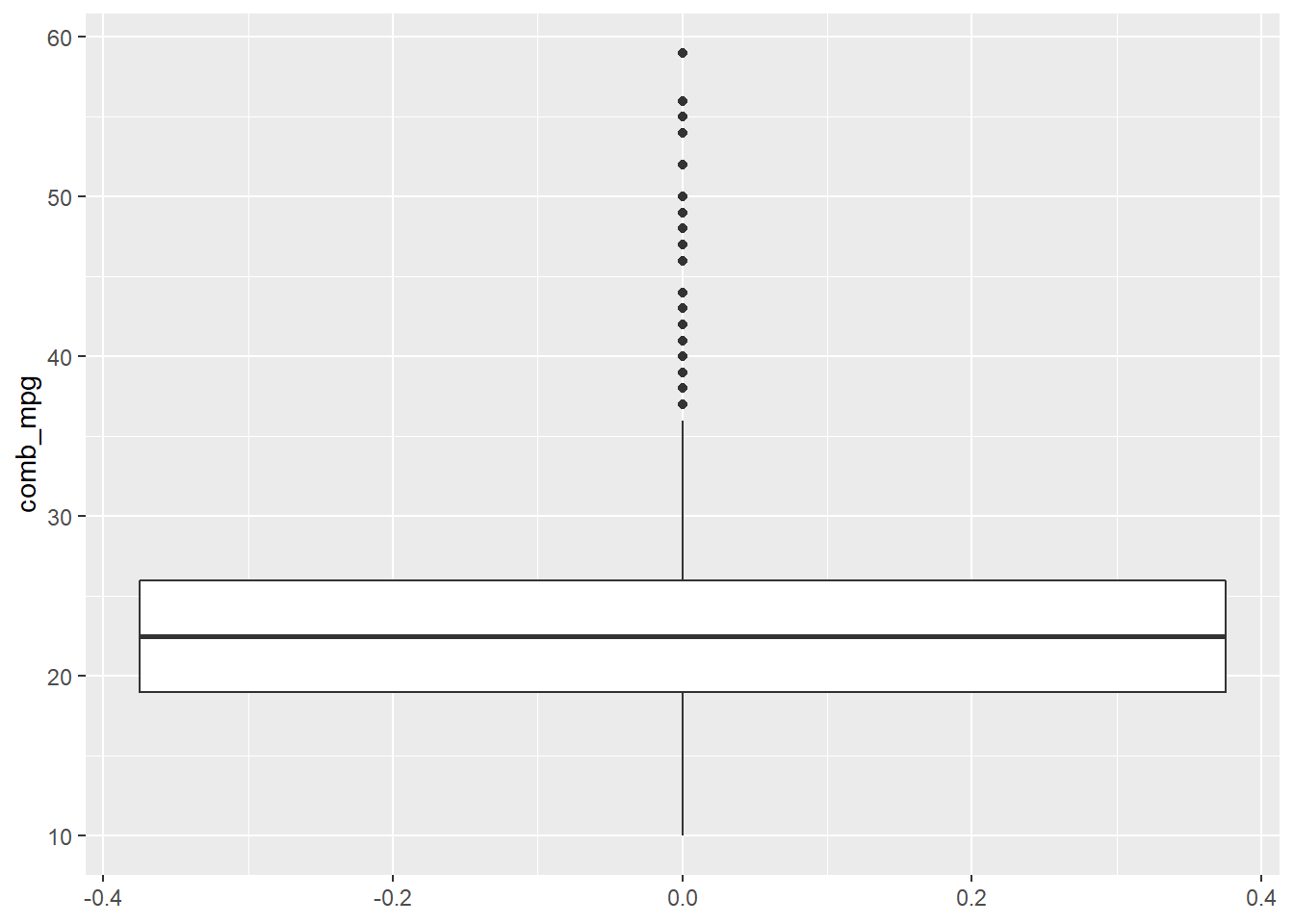
Inference for Proportions and Means
The following subsections illustrate the R commands for conducting a statistical hypothesis test for a single proportion, a difference of proportions, a single mean, paired means, and a difference of two means. Only the syntax is illustrated, refer to the lectures for more context.
Single Proportion
prop.test(18,45,p=0.32,correct = FALSE)##
## 1-sample proportions test without continuity correction
##
## data: 18 out of 45, null probability 0.32
## X-squared = 1.3235, df = 1, p-value = 0.25
## alternative hypothesis: true p is not equal to 0.32
## 95 percent confidence interval:
## 0.2702489 0.5454815
## sample estimates:
## p
## 0.4To conduct the same test “by hand,” we use
n <- 45
p_hat <- 18/n
p0 <- 0.32
SE <- sqrt((p0*(1-p0))/n)
(z_val <- (p_hat-p0)/SE )
## [1] 1.150447(p_val <- 2*(1-pnorm(z_val))) # since 2-sided and z_val > 0## [1] 0.2499596Difference of Proportions
prop.test(c(18,15),c(45,27),correct=FALSE)##
## 2-sample test for equality of proportions without continuity correction
##
## data: c(18, 15) out of c(45, 27)
## X-squared = 1.6448, df = 1, p-value = 0.1997
## alternative hypothesis: two.sided
## 95 percent confidence interval:
## -0.39138965 0.08027854
## sample estimates:
## prop 1 prop 2
## 0.4000000 0.5555556To conduct the same test “by hand,” we use
n1 <- 45
n2 <- 27
p_hat1 <- 18/n1
p_hat2 <- 15/n2
p_pooled <- (p_hat1*n1 + p_hat2*n2)/(n1+n2)
SE <- sqrt((p_pooled*(1-p_pooled))/n1 + (p_pooled*(1-p_pooled))/n2)
(z_val <- (p_hat1-p_hat2)/SE)
## [1] -1.28248(p_val <- 2*pnorm(z_val)) # since 2-sided and z_val < 0 ## [1] 0.1996743Single Mean
sim_data <- tibble(x=rnorm(18,2,0.75),y=rnorm(18,2.2,0.75))

t.test(sim_data$x,mu=1)
##
## One Sample t-test
##
## data: sim_data$x
## t = 4.9179, df = 17, p-value = 0.0001302
## alternative hypothesis: true mean is not equal to 1
## 95 percent confidence interval:
## 1.414160 2.036512
## sample estimates:
## mean of x
## 1.725336To conduct this test “by hand”, use
n <- length(sim_data$x)
mu_x <- mean(sim_data$x)
sd_x <- sd(sim_data$x)
SE <- sd_x/sqrt(n)
mu0 <- 1
(t_val <- (mu_x-mu0)/SE)
## [1] 4.917873(p_val <- 2*(1-pt(t_val,df=n-1))) # since 2-sided and t_val > 0## [1] 0.0001301682Paired Samples
t.test(sim_data$x,sim_data$y,paired = TRUE)##
## Paired t-test
##
## data: sim_data$x and sim_data$y
## t = -1.2347, df = 17, p-value = 0.2337
## alternative hypothesis: true mean difference is not equal to 0
## 95 percent confidence interval:
## -0.6445010 0.1686316
## sample estimates:
## mean difference
## -0.2379347To conduct this test “by hand”, use
xy_diff <- sim_data$x - sim_data$y
n <- length(xy_diff)
mu_diff <- mean(xy_diff)
sd_diff <- sd(xy_diff)
SE <- sd_diff/sqrt(n)
(t_val <- mu_diff/SE)
## [1] -1.234727(p_val <- 2*pt(t_val,df=n-1)) # since 2-sided and t_val < 0## [1] 0.2337271Difference of Means
z <- rnorm(22,2,0.75)

t.test(sim_data$x,z,paired=FALSE)
##
## Welch Two Sample t-test
##
## data: sim_data$x and z
## t = 0.91667, df = 37.426, p-value = 0.3652
## alternative hypothesis: true difference in means is not equal to 0
## 95 percent confidence interval:
## -0.2292265 0.6082575
## sample estimates:
## mean of x mean of y
## 1.725336 1.535820To do this test “by hand”, use
n1 <- length(sim_data$x)
n2 <- length(z)
mu_1 <- mean(sim_data$x)
sd_1 <- sd(sim_data$x)
mu_2 <- mean(z)
sd_2 <- sd(z)
mu_diff <- mu_1 - mu_2
SE <- sqrt(sd_1^2/n1 + sd_2^2/n2)
(t_val <- (mu_diff)/SE)
## [1] 0.9166679(p_val <- 2*(1-pt(t_val,df=min(n1-1,n2-1)))) # since 2-sided and t_val > 0## [1] 0.3721383Note: The results are slightly different from what
we see with the t.test command. This is due to the fact
that the t.test implementation utilizes a pooled standard
deviation which is a special topic that we did not cover in lecture.
Summary Stats for a Categorical Variable
For a single categorical variable, a one-way table is used to summarize the counts for how many times each level of the variable occurs as an observation in the sample data. For example,
table(my_data$drive_desc)##
## 2-Wheel Drive, Front 2-Wheel Drive, Rear 4-Wheel Drive
## 264 276 180
## All Wheel Drive Part-time 4-Wheel Drive
## 358 30The addmargins command totals the counts.
addmargins(table(my_data$drive_desc))##
## 2-Wheel Drive, Front 2-Wheel Drive, Rear 4-Wheel Drive
## 264 276 180
## All Wheel Drive Part-time 4-Wheel Drive Sum
## 358 30 1108Instead of counts, we can also compute proportions.
proportions(table(my_data$drive_desc))##
## 2-Wheel Drive, Front 2-Wheel Drive, Rear 4-Wheel Drive
## 0.23826715 0.24909747 0.16245487
## All Wheel Drive Part-time 4-Wheel Drive
## 0.32310469 0.02707581or with the total
addmargins(proportions(table(my_data$drive_desc)))##
## 2-Wheel Drive, Front 2-Wheel Drive, Rear 4-Wheel Drive
## 0.23826715 0.24909747 0.16245487
## All Wheel Drive Part-time 4-Wheel Drive Sum
## 0.32310469 0.02707581 1.00000000Visual Summaries for a Single Categorical Variable
A visualization that corresponds to a one-way table is provided by a bar plot.
gf_bar(~drive_desc,data=my_data)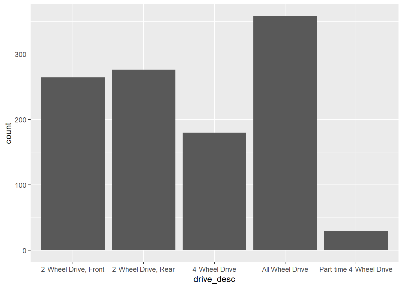
Note that the x-axis labels are difficult to read. This can be addressed as follows.
gf_bar(~drive_desc,data=my_data) +
  theme(axis.text.x = element_text(angle = 45, vjust = 1, hjust=1))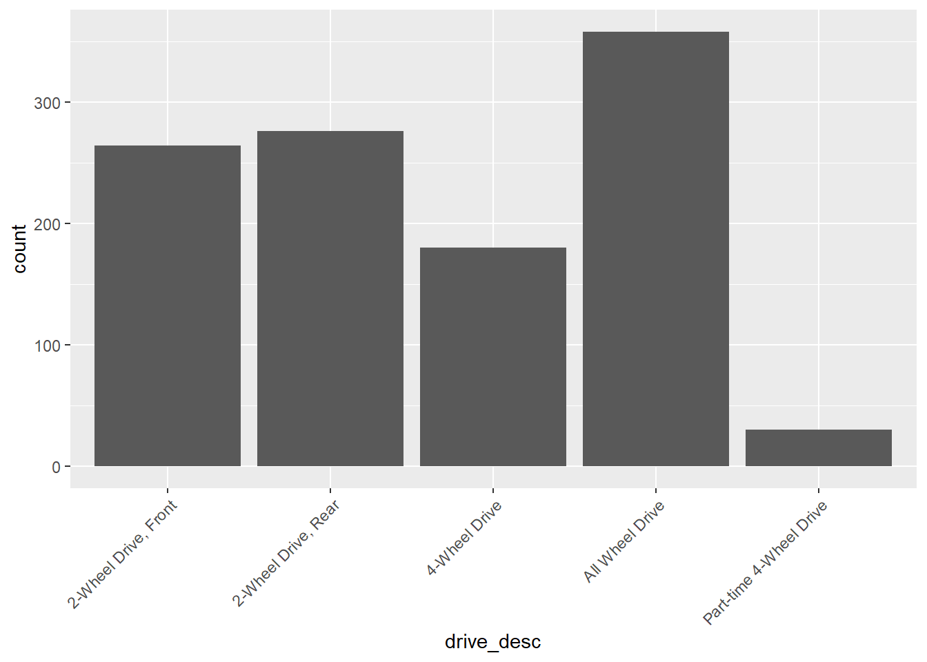
The proportions version of a bar plot is obtained with a mosaic plot.
ggplot(data = my_data) +
  geom_mosaic(aes(x = product(drive_desc), fill=drive_desc))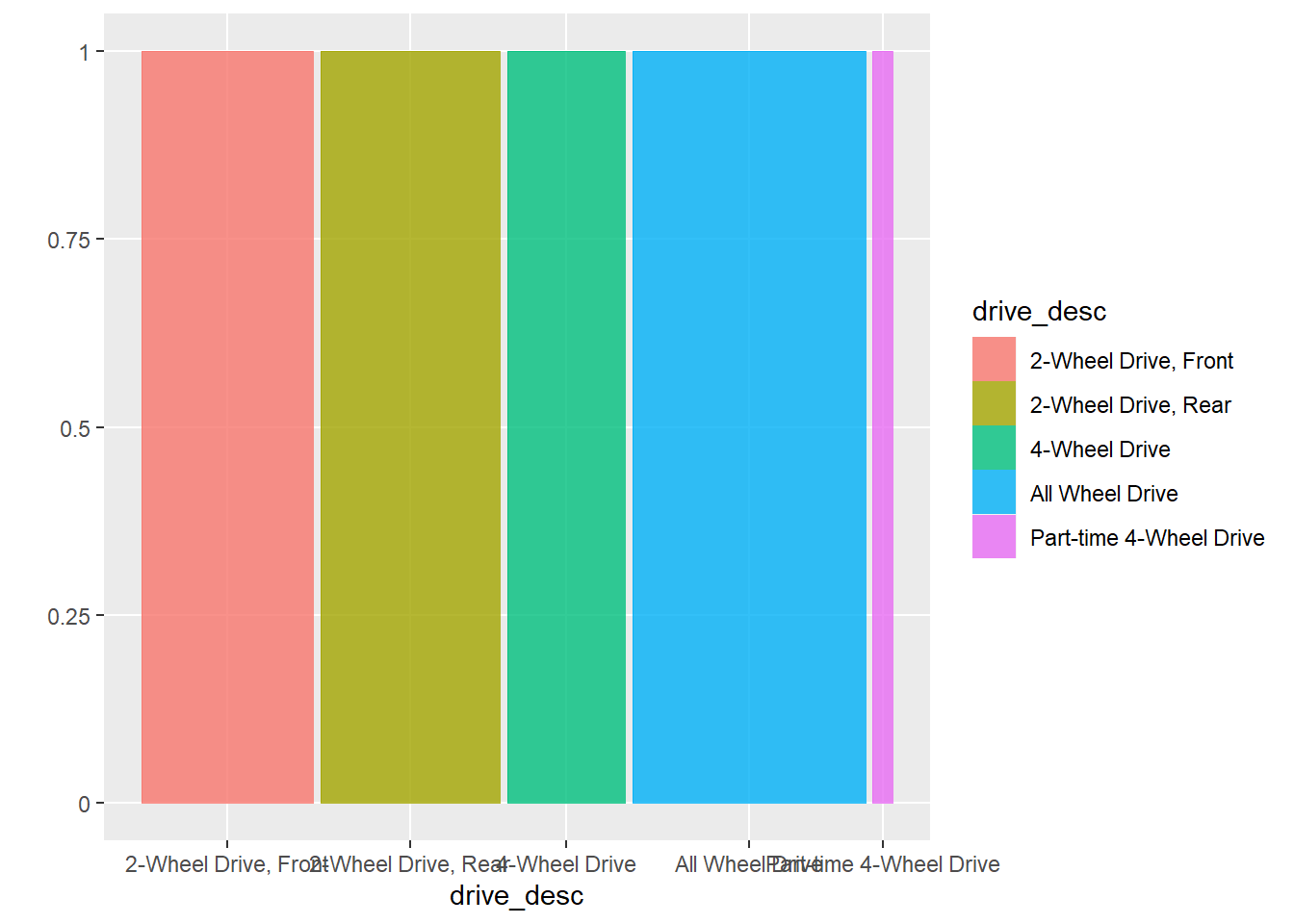
or with easier to read labeling:
ggplot(data = my_data) +
  geom_mosaic(aes(x = product(drive_desc), fill=drive_desc)) +
  theme(axis.text.x = element_text(angle = 45, vjust = 1, hjust=1))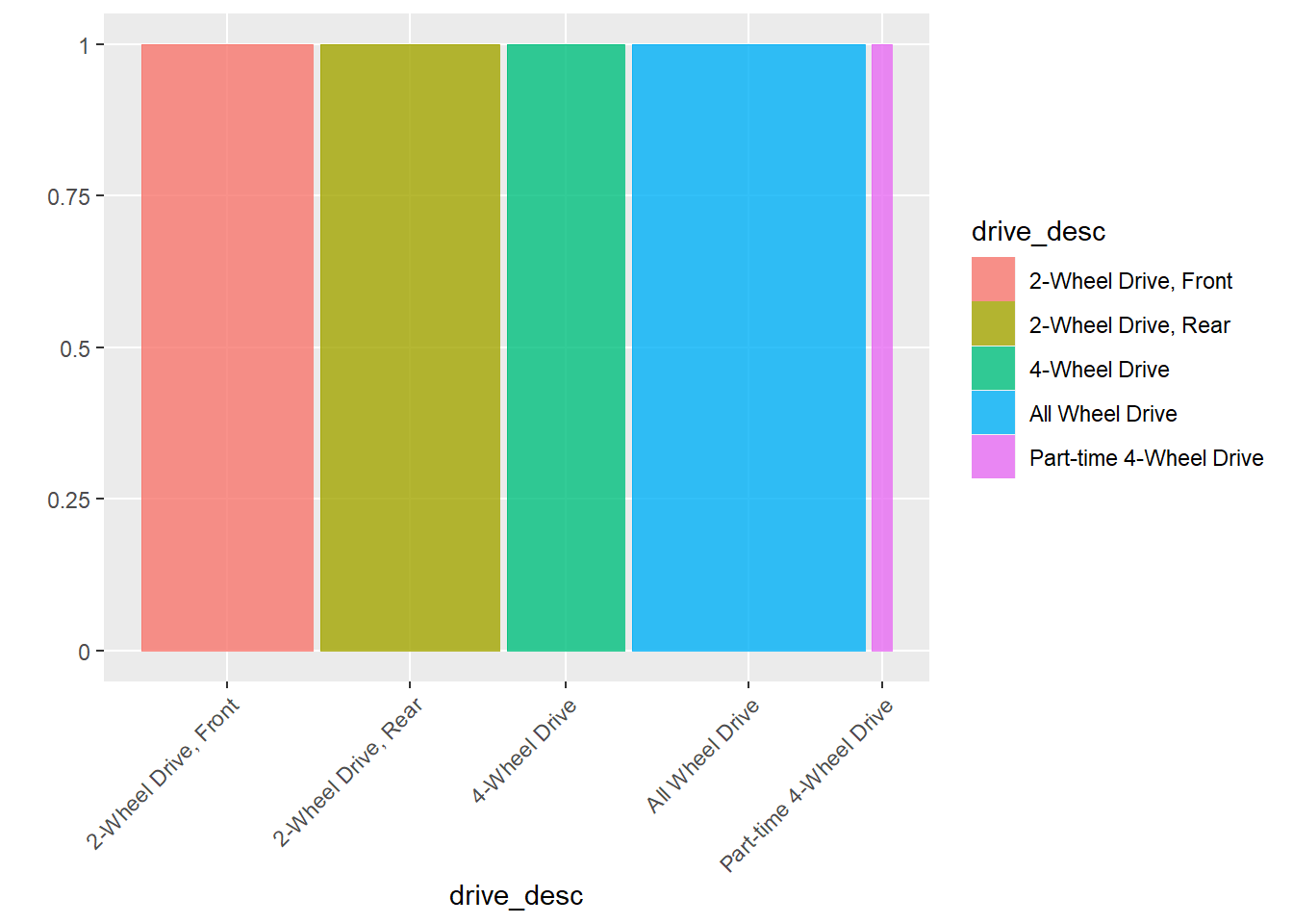
Variable Associations
Sometimes we are interested in the association of two variables. There are three typical situations:
Two numerical variables. To study this, we use correlation, scatter plots, and regression.
One numerical variable (as response) and one categorical variable (as explanatory). To study this, we use grouped summaries, side-by-side boxplots, and two-sample t-tests (when categorical variable is binary) or ANOVA.
Two categorical variables. Here, we use two-way tables, mosaic plots, and chi-square tests.
Two Numeric Variables
Consider for example, the variables comb_mpg (combined
mileage) and engine_displacement (engine displacement). We
may want to know if fuel efficiency is realted to engine size.
The correlation of these two variables is
(R_val <- cor(my_data$engine_displacement,my_data$comb_mpg))## [1] -0.7027217This value squared is \(R^2\):
R_val^2## [1] 0.4938177Let’s examine the scatter plot for these variables:
# scatterplot for two numerical variables
gf_point(comb_mpg~engine_displacement,data=my_data)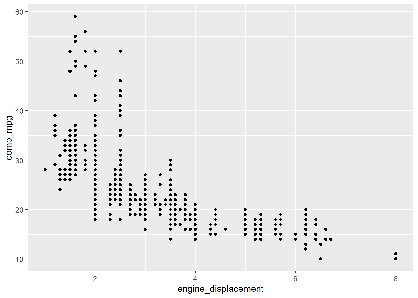
If we want to include the regression line, it can be added as follows:
gf_point(comb_mpg~engine_displacement,data=my_data) %>%
  gf_lm()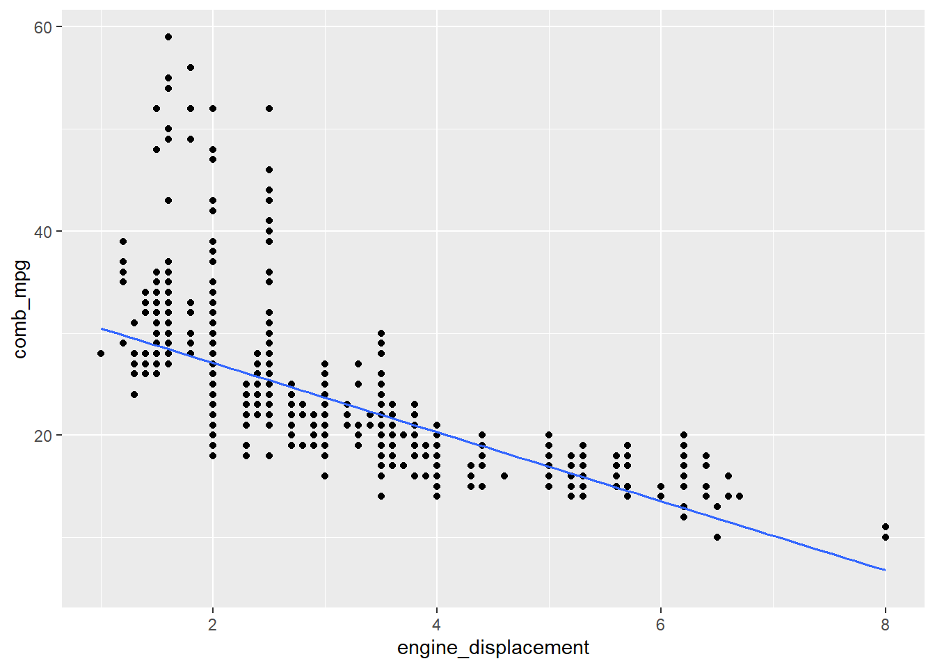
The following code fits a linear model for these variables and returns the inferential statistics:
lm_fit <- lm(comb_mpg~engine_displacement,data=my_data)
summary(lm_fit)
##
## Call:
## lm(formula = comb_mpg ~ engine_displacement, data = my_data)
##
## Residuals:
## Min 1Q Median 3Q Max
## -9.0920 -2.7068 -0.7068 1.9080 30.5539
##
## Coefficients:
## Estimate Std. Error t value Pr(>|t|)
## (Intercept) 33.8624 0.3503 96.68 <2e-16 ***
## engine_displacement -3.3852 0.1031 -32.85 <2e-16 ***
## ---
## Signif. codes: 0 '***' 0.001 '**' 0.01 '*' 0.05 '.' 0.1 ' ' 1
##
## Residual standard error: 4.588 on 1106 degrees of freedom
## Multiple R-squared: 0.4938, Adjusted R-squared: 0.4934
## F-statistic: 1079 on 1 and 1106 DF, p-value: < 2.2e-16We can clean this output up using the commands from the
broom package. For example,
tidy(lm_fit)## # A tibble: 2 × 5
## term estimate std.error statistic p.value
## <chr> <dbl> <dbl> <dbl> <dbl>
## 1 (Intercept) 33.9 0.350 96.7 0
## 2 engine_displacement -3.39 0.103 -32.8 1.03e-165outputs the parameter estimates, standard errors, and p-values for
the intercept and slope parameters. The glance command
provides additional information such as the \(R^2\) value and the degrees of freedom
df.residual (notice that this is \(n-2\) where \(n\) is the number of observations).
glance(lm_fit)## # A tibble: 1 × 12
## r.squared adj.r.squared sigma statistic p.value df logLik AIC BIC
## <dbl> <dbl> <dbl> <dbl> <dbl> <dbl> <dbl> <dbl> <dbl>
## 1 0.494 0.493 4.59 1079. 1.03e-165 1 -3259. 6524. 6539.
## # … with 3 more variables: deviance <dbl>, df.residual <int>, nobs <int>Residual plots are very helpful to assess potential issues with a
linear fit. Here is code that produces a residual plot. Note that the
first step is to obtain the residuals using the augment
function.
lm_fit %>% augment() %>%
  gf_point(.resid~engine_displacement) %>% gf_hline(yintercept = 0,linetype="dashed")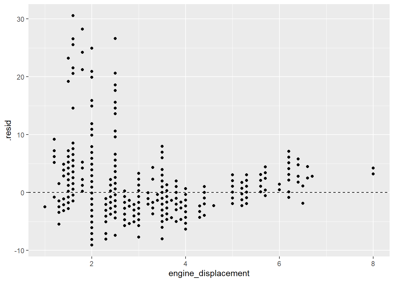
Note that the residuals are not evenly distributed around the 0 line which indicates that a linear model is not appropriate for this data.
Numerical Response and Categorical Explanatory
How does the distribution of a numerical variable depend on the category to which the samples belong? For example, how does the combined gas mileage depend on what kind of drive system a vehicle uses?
We can compute grouped summary statistics. For example, the mean gas mileage per class of drive system is computed as follows:
my_data %>% group_by(drive_desc) %>% summarise(mean_comb_mpg=mean(comb_mpg))## # A tibble: 5 × 2
## drive_desc mean_comb_mpg
## <chr> <dbl>
## 1 2-Wheel Drive, Front 29.9
## 2 2-Wheel Drive, Rear 20.6
## 3 4-Wheel Drive 20.0
## 4 All Wheel Drive 22.3
## 5 Part-time 4-Wheel Drive 21.3A side-by-side boxplot allows us to see the distribution of a numerical variable by category.
gf_boxplot(comb_mpg~drive_desc,data=my_data)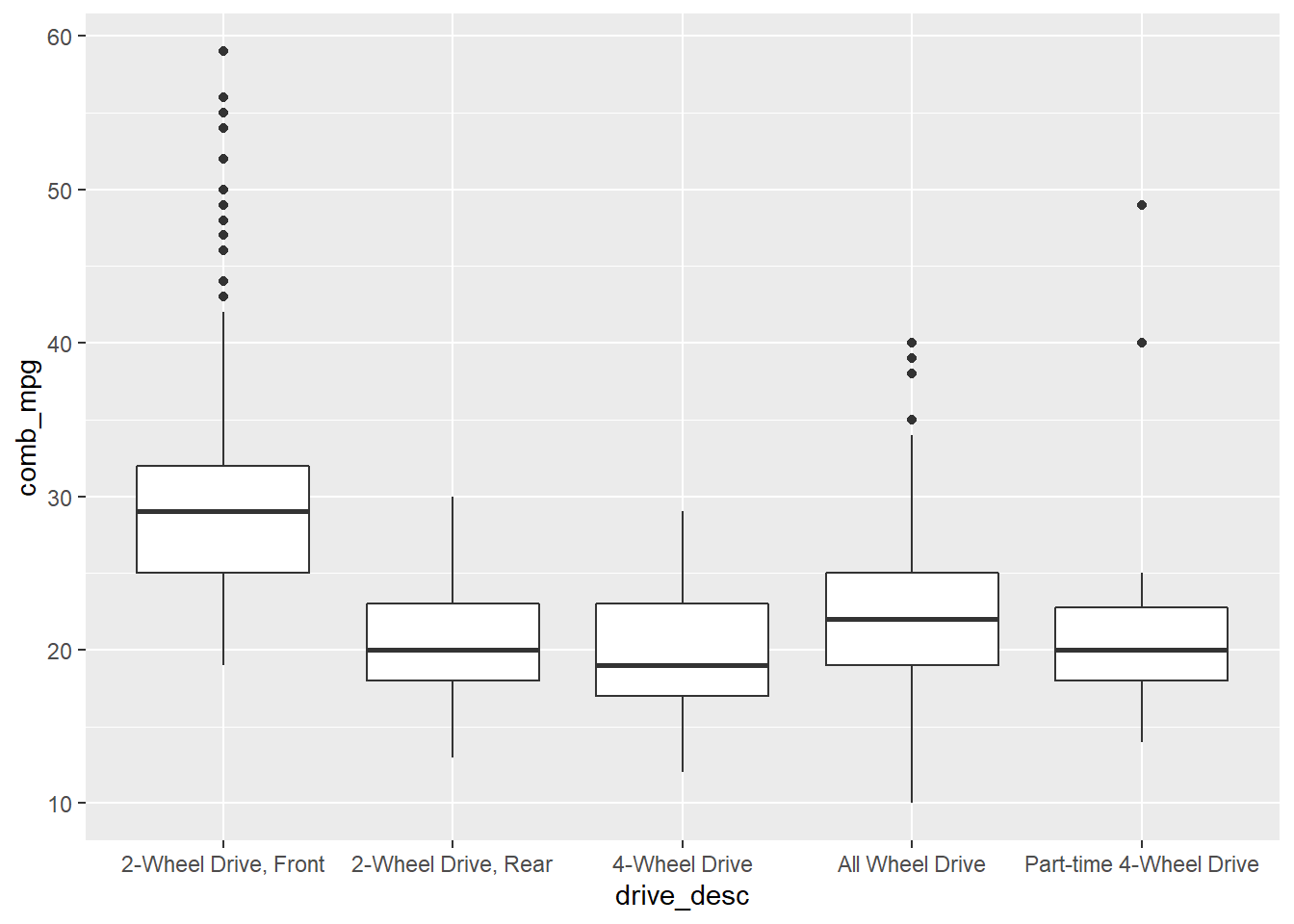
or
gf_boxplot(comb_mpg~drive_desc,data=my_data) +
  theme(axis.text.x = element_text(angle = 45, vjust = 1, hjust=1))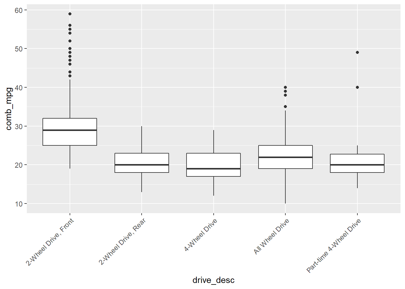
Inference with ANOVA
In order to test if the observed difference in means is likely true, or is simply a result of sampling, we use an ANOVA. This is conducted as follows:
summary(aov(comb_mpg~drive_desc,data=my_data))## Df Sum Sq Mean Sq F value Pr(>F)
## drive_desc 4 16025 4006 147.4 <2e-16 ***
## Residuals 1103 29970 27
## ---
## Signif. codes: 0 '***' 0.001 '**' 0.01 '*' 0.05 '.' 0.1 ' ' 1Association for a Pair of Categorical Variables
A two-way or cross table compares combinations of categories for two
categorical variables. For example, conside the data set
hsb2 from the openintro package which records
samples from the High School and Beyond survey, a survey conducted on
high school seniors by the National Center of Education Statistics.
table(hsb2$ses,hsb2$prog)##
## general academic vocational
## low 16 19 12
## middle 20 44 31
## high 9 42 7We can also add the margin sum totals
addmargins(table(hsb2$ses,hsb2$prog))##
## general academic vocational Sum
## low 16 19 12 47
## middle 20 44 31 95
## high 9 42 7 58
## Sum 45 105 50 200Here ses is the socio economic status of student’s
family and prog is the type of program.
A mosaic plot can be used to visualize this data.
ggplot(data = hsb2) +
  geom_mosaic(aes(x = product(ses, prog), fill=ses)) +
  theme(axis.text.x = element_text(angle = 45, vjust = 1, hjust=1))
## Warning: `unite_()` was deprecated in tidyr 1.2.0.
## Please use `unite()` instead.
## This warning is displayed once every 8 hours.
## Call `lifecycle::last_lifecycle_warnings()` to see where this warning was generated.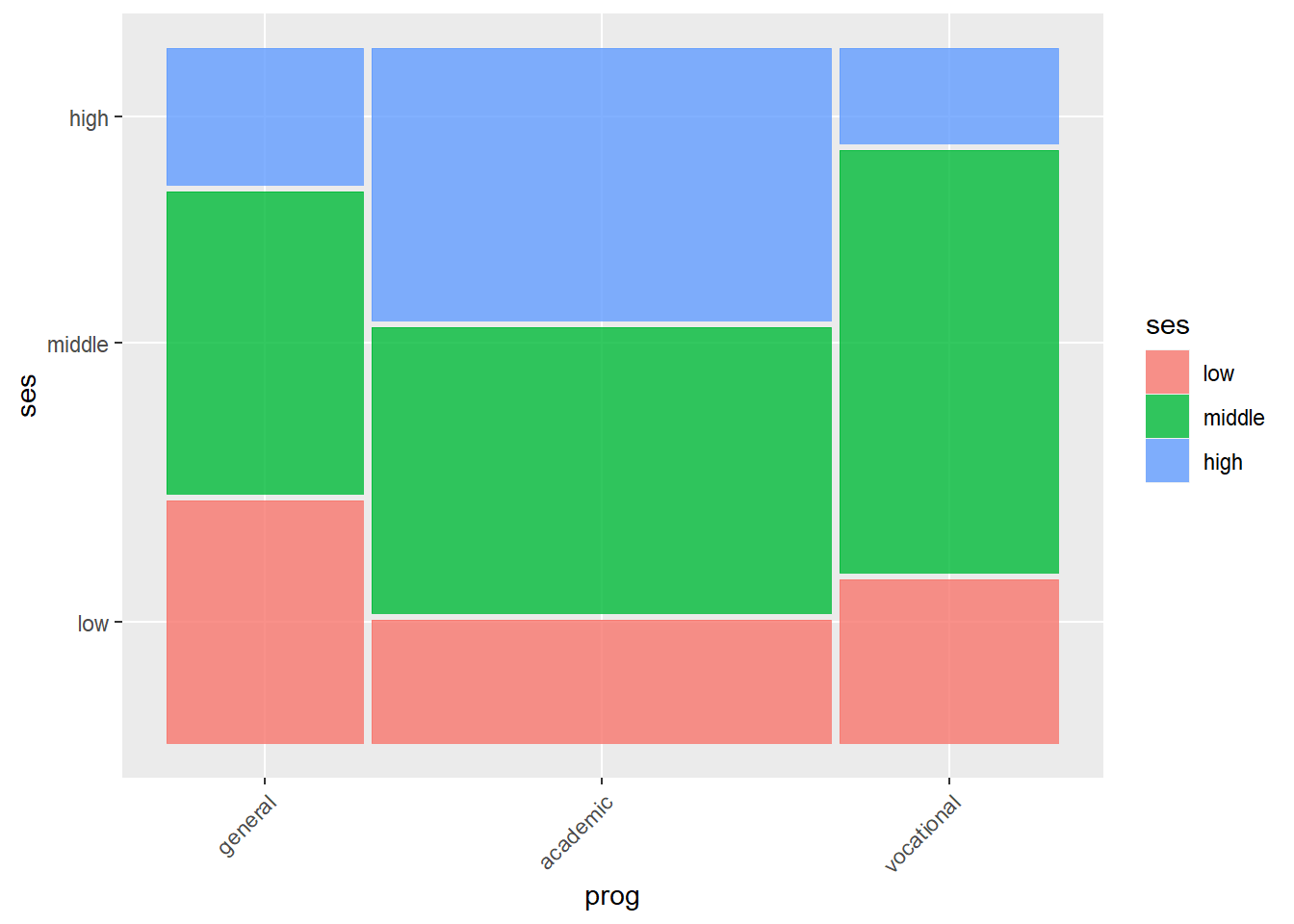
Inference with chi-square
We can ask if the variables ses and prog
are independent. A chi-square test helps to answer this.
chisq.test(hsb2$ses,hsb2$prog)##
## Pearson's Chi-squared test
##
## data: hsb2$ses and hsb2$prog
## X-squared = 16.604, df = 4, p-value = 0.002307Working with Distributions.
In order to conduct hypothesis test “by hand”, it helpful to be able to work with the basic distribution functions in R. For each distribution there are four functions:
r_dist_namewhich draws random samplesd_dist_namewhich represents the density function or probability mass functionp_dist_namewhich represents the cumulative distribution function, this is used to compute left-tail areasq_dist_nameis the quantile function which is the inverse function ofp_dist_name
Suppose for example that we want to work with a normal distribution.
Then we replace _dist_name with norm. For
example,
(sim_x <- rnorm(75,10,2.5))## [1] 14.014774 7.105479 11.641471 16.372478 9.913099 8.325916 9.980988
## [8] 14.442711 7.153481 13.419568 13.323912 10.841182 10.017232 8.861328
## [15] 9.083690 11.620716 15.175677 9.616504 6.523248 8.191046 10.645654
## [22] 9.207352 9.555525 9.575015 6.569245 9.565532 12.125581 11.744022
## [29] 11.374993 8.993170 9.521016 7.013680 9.867103 10.637990 14.264910
## [36] 12.503783 8.761041 10.888876 7.163480 12.195509 12.432292 15.302793
## [43] 11.036309 8.813204 10.164984 8.743806 7.935004 10.417473 7.759338
## [50] 10.420463 10.887421 9.869737 9.510163 8.377326 7.225582 12.123186
## [57] 10.055906 12.077852 6.889280 10.422566 11.682916 9.934309 9.521520
## [64] 8.045233 15.145405 11.876254 14.560521 10.200149 8.421477 6.216780
## [71] 8.409750 10.565754 12.534226 10.631875 7.070129Let’s make a histogram of this data:
gf_histogram(~sim_x,binwidth = 1.0,color="black")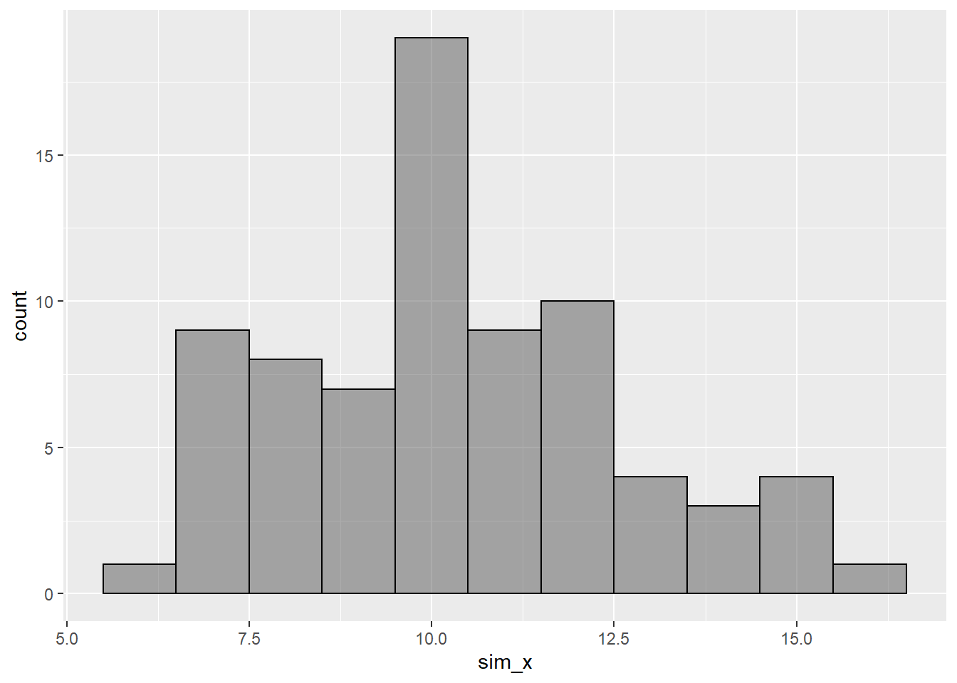
Here are illustrations of the uses of the other distribution functions:
The value of the standard normal density function at \(z=0\) is
dnorm(0.0)## [1] 0.3989423Let’s plot the standard normal density curve:
gf_dist("norm")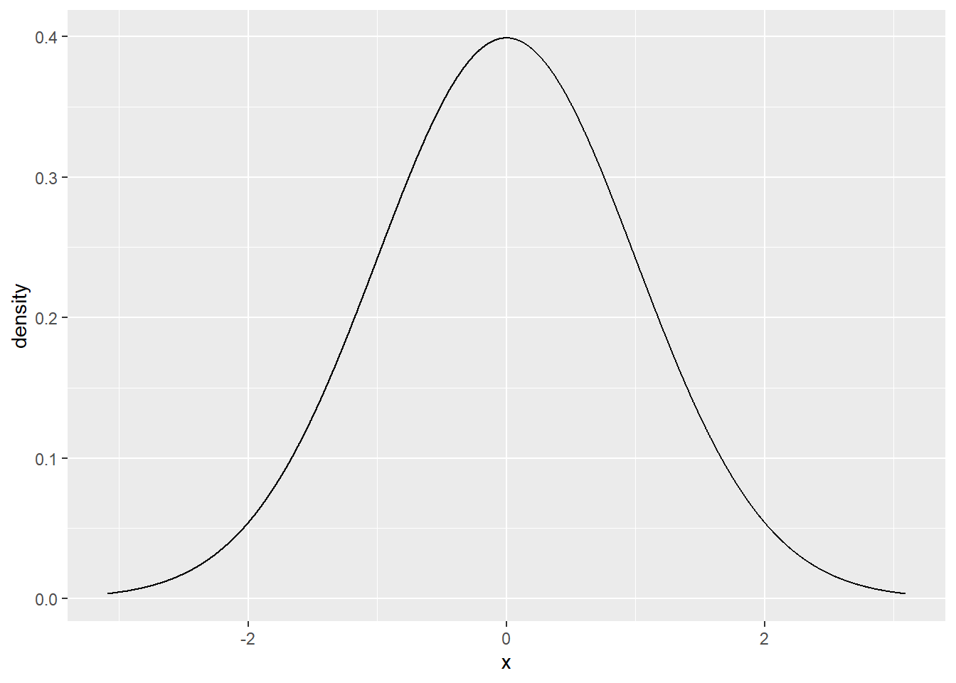
The use of the p and q functions are
illustrated with
pnorm(1.5)## [1] 0.9331928and
qnorm(0.3)## [1] -0.5244005Note Depending on the type of distribution you want
to work with, you need to specify appropriate values for an parameters.
For example, to work with a t distribution to need to specify the
appropriate values for the degrees of freedom df.
Two Bonus Commands
Data Summary with skim
An even fancier summary of our data is provided by the
skim function from the skimr package. Let’s
see how it works.
skimr::skim(my_data)| Name | my_data |
| Number of rows | 1108 |
| Number of columns | 28 |
| _______________________ | |
| Column type frequency: | |
| character | 20 |
| numeric | 8 |
| ________________________ | |
| Group variables | None |
Variable type: character
| skim_variable | n_missing | complete_rate | min | max | empty | n_unique | whitespace |
|---|---|---|---|---|---|---|---|
| mfr_name | 0 | 1.00 | 3 | 20 | 0 | 22 | 0 |
| division | 0 | 1.00 | 3 | 32 | 0 | 41 | 0 |
| carline | 0 | 1.00 | 2 | 32 | 0 | 788 | 0 |
| mfr_code | 0 | 1.00 | 3 | 3 | 0 | 22 | 0 |
| transmission_speed | 0 | 1.00 | 8 | 12 | 0 | 25 | 0 |
| guzzler | 0 | 1.00 | 1 | 1 | 0 | 2 | 0 |
| air_aspir_method | 439 | 0.60 | 2 | 2 | 0 | 4 | 0 |
| air_aspir_method_desc | 0 | 1.00 | 5 | 25 | 0 | 5 | 0 |
| transmission | 0 | 1.00 | 1 | 3 | 0 | 7 | 0 |
| transmission_desc | 0 | 1.00 | 6 | 65 | 0 | 7 | 0 |
| trans_lockup | 0 | 1.00 | 1 | 1 | 0 | 2 | 0 |
| trans_creeper_gear | 0 | 1.00 | 1 | 1 | 0 | 2 | 0 |
| drive_sys | 0 | 1.00 | 1 | 1 | 0 | 5 | 0 |
| drive_desc | 0 | 1.00 | 13 | 23 | 0 | 5 | 0 |
| fuel_usage | 0 | 1.00 | 1 | 3 | 0 | 6 | 0 |
| fuel_usage_desc | 0 | 1.00 | 28 | 42 | 0 | 6 | 0 |
| class | 0 | 1.00 | 10 | 36 | 0 | 22 | 0 |
| car_truck | 507 | 0.54 | 1 | 3 | 0 | 3 | 0 |
| release_date | 0 | 1.00 | 20 | 20 | 0 | 159 | 0 |
| fuel_cell | 856 | 0.23 | 1 | 1 | 0 | 1 | 0 |
Variable type: numeric
| skim_variable | n_missing | complete_rate | mean | sd | p0 | p25 | p50 | p75 | p100 | hist |
|---|---|---|---|---|---|---|---|---|---|---|
| model_yr | 0 | 1 | 2021.00 | 0.00 | 2021 | 2021 | 2021.0 | 2021.0 | 2021 | ▁▁▇▁▁ |
| model_type_index | 0 | 1 | 259.36 | 271.47 | 1 | 40 | 114.0 | 507.0 | 999 | ▇▂▂▂▁ |
| engine_displacement | 0 | 1 | 3.12 | 1.34 | 1 | 2 | 3.0 | 3.8 | 8 | ▇▇▂▂▁ |
| no_cylinders | 0 | 1 | 5.60 | 1.92 | 3 | 4 | 6.0 | 6.0 | 16 | ▇▇▁▁▁ |
| city_mpg | 0 | 1 | 20.89 | 6.60 | 8 | 17 | 20.0 | 23.0 | 58 | ▆▇▁▁▁ |
| hwy_mpg | 0 | 1 | 27.30 | 6.42 | 13 | 23 | 27.0 | 31.0 | 60 | ▃▇▃▁▁ |
| comb_mpg | 0 | 1 | 23.29 | 6.45 | 10 | 19 | 22.5 | 26.0 | 59 | ▃▇▂▁▁ |
| no_gears | 0 | 1 | 7.50 | 1.87 | 1 | 6 | 8.0 | 8.0 | 10 | ▁▁▃▇▃ |
Essentially what this shows is that we have 20 categorical variables
and 8 numerical variables. For each of the numerical variables, the
skim function reports all of the quantitative summary
statistic values.
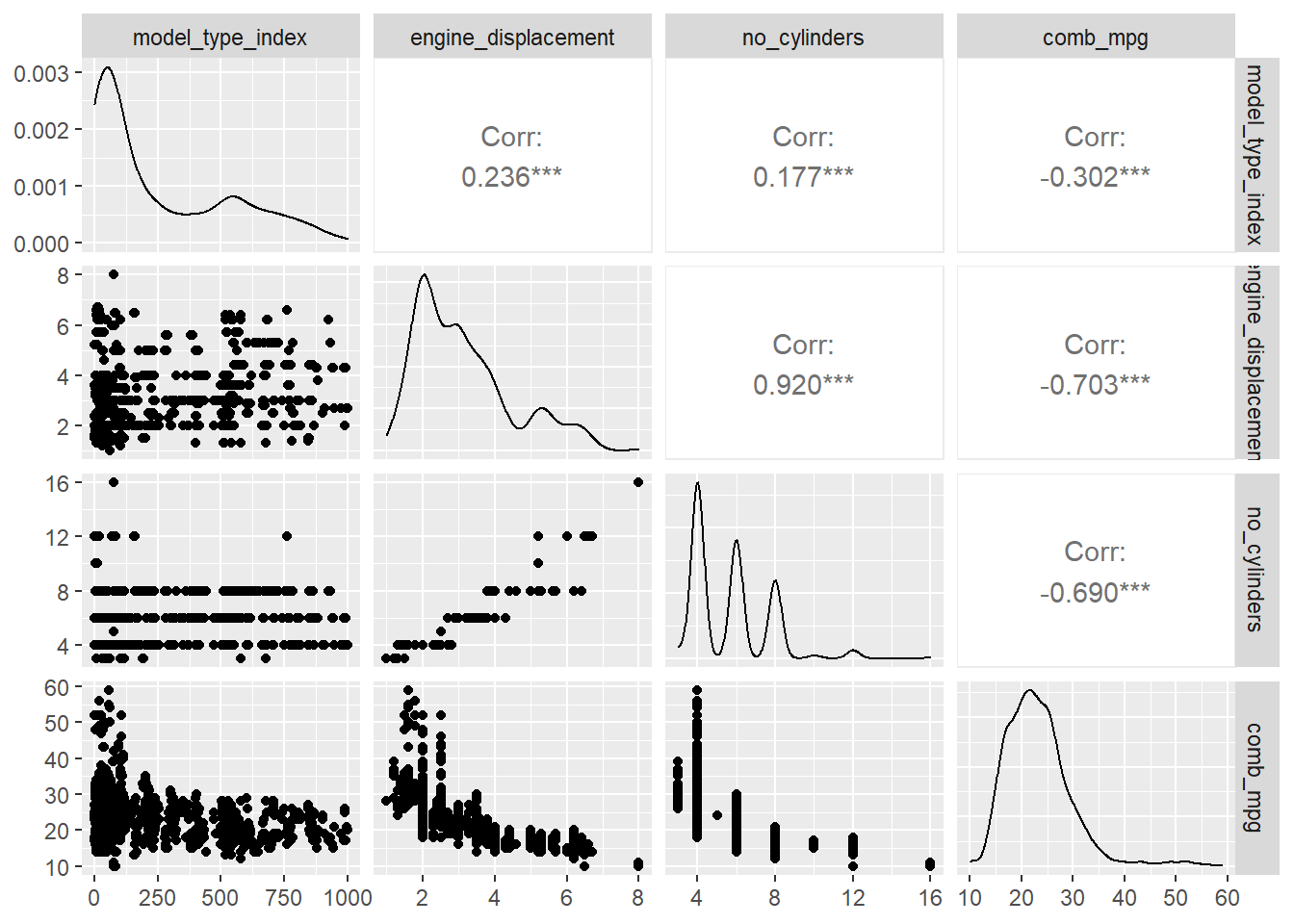
Mulitple Scatter Plots with ggpairs
We might want to study the associations of multiple numerical
variables simultaneously. The ggpairs command from the
GGally package is a way to obtain a lot of information
about several numerical varaibles with one plot. For example,
GGally::ggpairs(my_data[,c(6,7,8,12)])